# Global Flood Monitoring

The Global Flood Monitoring (GFM) product is a component of the EU’s Copernicus Emergency Management Service (CEMS) that provides continuous monitoring of floods worldwide, by processing and analysing in near real-time all incoming Sentinel-1 SAR acquisitions over land.

The operational implementation the GFM product includes the following key elements:

Downloading of worldwide Sentinel-1 SAR acquisitions (Level-1 IW GRDH)
Pre-processing of the downloaded Sentinel-1 data to backscatter data (SIG0)
Operational application of three fully automated flood mapping algorithms.
An ensemble-based approach is then used to combine the three flood extent outputs of the individual flood algorithms.
Generation of the required GFM output layers, including Observed flood extent, Reference water mask, Exclusion Mask and Likelihood Values.
Web service-based access and dissemination of the GFM product output layers.

# Output layers used in openEO

Observed flood extent (ENSEMBLE of all three individual flood outputs)
Reference water mask (permament and seasonal water bodies)

# Links

https://extwiki.eodc.eu/GFM

# Compute the maximum flood extent

In this example, we have a closer look at an area in Pakistan, which was ravaged by the unprecedented floods of 2022. The flooding caused severe damage and economic losses and is referred to as the worst flood in the history of Pakistan. We compute the sum of flooded pixels over time.

import openeo
from openeo.processes import *

backend = "openeo.cloud"
conn = openeo.connect(backend).authenticate_oidc()

spatial_extent  = {'west': 67.5, 'east': 70, 'south': 24.5, 'north': 26}
temporal_extent = ["2022-09-01", "2022-10-01"] 
collection      = 'GFM'

gfm_data = conn.load_collection(
    collection, 
    spatial_extent=spatial_extent, 
    temporal_extent=temporal_extent, 
    bands = ["flood_extent"]
)
gfm_sum = gfm_data.reduce_dimension(dimension="t", reducer=sum)

gfm_sum_tiff = gfm_sum.save_result(format="GTiff", options={"tile_grid": "wgs84-1degree"})

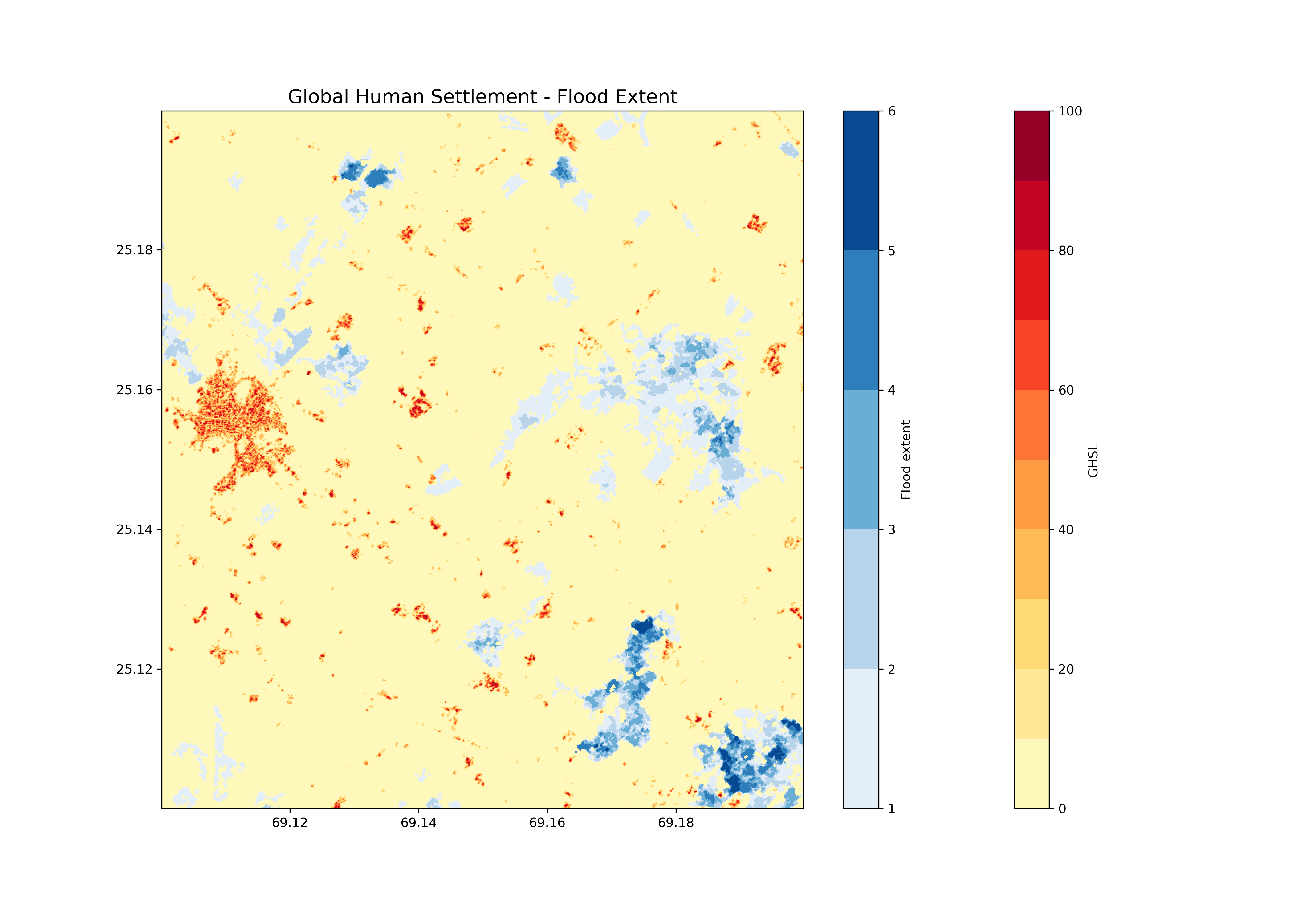
# Explore how the flood extent relates to the Global Human Settlement Built-up layer

We display the flood extent next to the Global Human Settlement Built-up layer.

The Global Human Settlement Layer (GHSL) project produces global spatial information about the human presence on the planet over time in the form of built-up maps, population density maps and settlement maps.

Here, the GHS-BUILT-S spatial raster dataset at 10m resolution is used which depicts the distribution of built-up surfaces, expressed as number of square metres.

Values are between 0 and 100 and represent the amount of square metres of built-up surface in the cell.

https://ghsl.jrc.ec.europa.eu/about.php

The GHSL is available in wgs84. Therefore, the tile_grid for the GFM data was set to wgs84 as well.

Flood extent — Figure 1: Estimate of how the built-up surface was effected by the flood in Pakistan in September 2022. Some of the highest values of the GHSL can be found around 25.16 N 69.11 E, which marks Digri Tehsil, the second largest town of Mirpurkhas District, Pakistan.

# Statistical analysis

In the example given above, we picked the sum in gfm_sum = gfm_data.reduce_dimension(dimension="t", reducer=sum). OpenEO provides a range of reducers to choose from. E.g.:

Compute the flood frequency: set the reducer to mean
Generate the mask of flooded pixels: set the reducer to any

gfm_flood_frequency = gfm_data.reduce_dimension(dimension="t", reducer=mean)

gfm_flood_frequency_tiff = gfm_flood_frequency.save_result(format="GTiff", options={"tile_grid": "wgs84-1degree"})

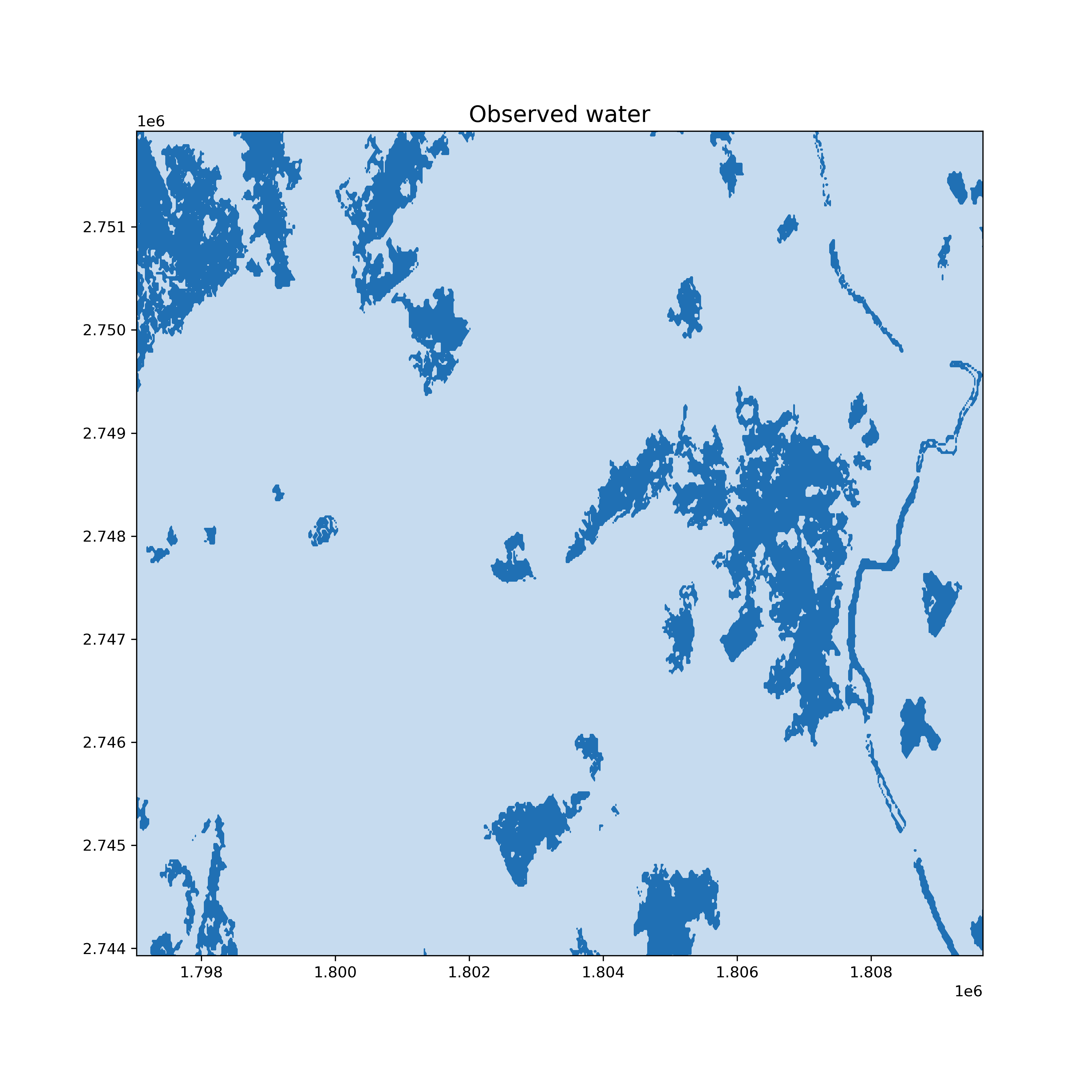
# Observed water (flood_extent + refwater)

The observed water combines both flood extent and the reference water mask. The reference water mask represents permanent or seasonal water bodies, which are clearly distinct from flood events. With openEO, the two layers flood_extent and refwater can be combined directly and stored into one file. No need to download layers individually.

spatial_extent  = {'west': 67.5, 'east': 70, 'south': 24.5, 'north': 26}
temporal_extent = ["2022-09-01", "2022-10-01"] 
collection      = 'GFM'

gfm_data = conn.load_collection(
    collection, 
    spatial_extent=spatial_extent, 
    temporal_extent=temporal_extent, 
    bands = ["flood_extent", "refwater"]
)

# retrieve all pixels which have been detected as water during the given period
# -> observed water
observed_water = gfm_data.reduce_dimension(dimension="bands", reducer=any).reduce_dimension(dimension="t", reducer=any)

# Save the result in Equi7Grid and as GeoTiff
observed_water_tif = observed_water.save_result(format="GTiff", options={"tile_grid": "equi7"})

# Explore the observed water

The original GFM data is stored in the Equi7 Grid and the Asian Equi7 coordinate reference system. With the tile_grid parameter, the user can either keep the data like this, or pick a different CRS.