# Crop Classification

The goal of this section is to show how openEO functionality can be integrated into a basic feature engineering pipeline. We will do this using crop classification as an example.

The constantly increasing demand of food has resulted in a highly intensified agricultural production. This intensification on the one hand requires more planning and management, and on the other, threatens ecosystem services that need to be monitored by scientists and decision makers who rely on detailed spatial information of crop cover in agricultural areas.

Crop classification on a large scale is a challenging task, but with the recent advances in satellite sensor technology and the push of a.o. the ESA for higher resolution open satellite data with a frequent revisit time this task has become possible.

There are various approaches to crop classification. One can use basic rule-based classification, or use more sophisticated methods such as one of various machine learning models. In this example, we will show both of these approaches.

Generally, any classification task will contain the following steps:

(1) Preprocessing & feature engineering
(2) Training
(3) Classification & model evaluation

We will have a more detailed look at all three of these steps, and provide code examples along the way.

To see a fully working example, you can check out this Python notebook on rule-based classification (opens new window) or this Python notebook on classification using Random Forest (opens new window).

cropcover_closeup

# Preprocessing & feature engineering

Feature engineering refers to extracting a number of discriminative features from a single pixel timeseries or even a time series of EO data tiles. These features can in turn be used for any type of classification, ranging from an expert rule-based decision approach to regular machine learning techniques such as random forest or deep learning techniques based on neural networks.

Concrete examples of such features include basic statistics such as the percentiles or standard deviation of a vegetation index or the mean band value for given month, but can also be more complex such as derivatives of phenology or texture.

In general, data scientists like to explore the usefulness of a given feature set for a use case, or may even define new features. In some cases, the openEO processes will allow computing them, and in others, a 'user defined function' may be used to compute features that are not directly supported in openEO.

# Data preparation

To correctly compute and use statistics over a timeseries, we need gap-free composites at fixed timesteps. The goal of temporal aggregation is to create these gap-free composites at equidistant temporal intervals. This is especially true in the case of optical data, which is often cloudmasked before this step, introducing a lot of gaps ("no-data" values).

Example:

# Computing temporal features

For this use case, we will fully reduce the temporal dimension per band by calculating a number of stastics. These stastics are three quantiles, the mean and the standard deviation for each band. After computing the actual features, we have to make sure to rename the bands to reflect what has been calculated.

The effect of setting target_dimension to bands is that the 'time' dimension is removed, and replaced by the 'bands' dimension. We will use this same procedure to do band math on temporal features in the chapter "Rule-based classification".

Now, a complete datacube with features is available for further usage.

# Model training

Crop classification is generally tackled using a form of supervised learning, which requires a set of features with their respective labels. These labels often come in the form of labeled field polygons, however these polygons do not contain any of the features that your model might require. They need to be extracted from the DataCube that you created in the previous section.

In OpenEO, we can perform feature point/polygon extraction using the parameter sample_by_feature=True.

This will write the features of DataCube features of every point in barley_points to a separate netCDF file. Next we can read in all of these features with their respective label in a pandas dataframe, which can subsequently used for training. Training a model happens outside of openEO and will therefore not be explained in detail here, but you can have a look at the random forest notebook if that is something you need help with.

# Classification

# Rule-based classification

A simple approach is to define rules based on your features to classify crops. For example, when looking at temporal profiles of corn, we can see that the NDVI of may is smaller than the NDVI of june. By creating and iteratively refining rules for each of these crop types, we can get a first classification result.

However, to do this, we need to be able to do band math on the temporal dimension. Remember target_dimension="bands" that we used before to calculate the statistics over the temporal dimension? We can use this again to stack the temporal dimension onto the band dimension.

Next, we can do boolean comparison of features and see whether any given pixel matches the rules you determined.

Each of these rules results in a boolean that can be combined using geometric progression, to obtain a final cube containing all crop type predictions.

# Supervised classification using Random Forest

A more sophisticated approach is to use a machine learning model such as Random Forest. As mentioned before, training is done after feature extraction outside of openEO, and you can then pickle your model and store it on a repository. Next, you define a UDF that unpickles your model, predicts, and returns a new DataCube instance that contains the predicted values instead of the features.

Note that if your labels are strings, you will have to map them to integers. You can then download the classification results and plot it. Congratulations!

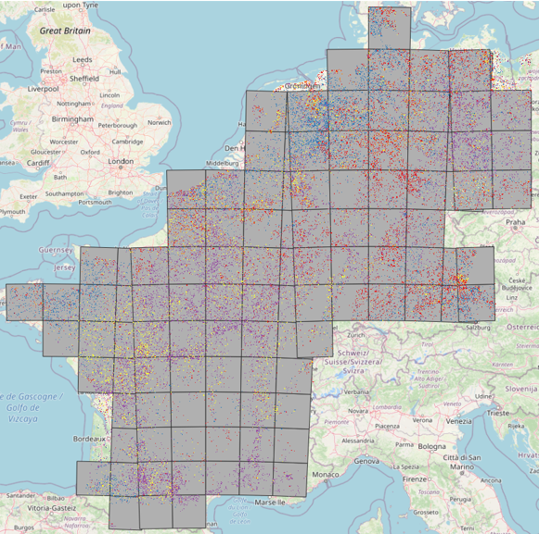
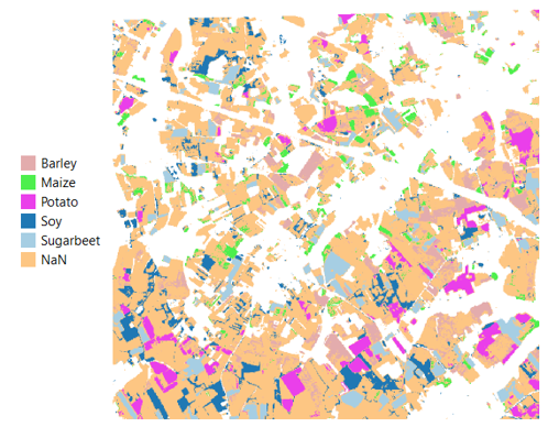
We ran the code in that notebook for ~120 MGRS tiles to end up with a crop cover map for 5 countries in Europe, which looks like this:

cropcover_5_countries