# Crop conditions
Attention
To use this service, you have to be registered at openEO platform. If you are not yet registered, you can apply here (opens new window).
To enable higher time-series resolution vegetation indices (such as NDVI, LAI, FAPAR, FCOVER) than the Sentinel-2 time series, we have implemented the computation based on the Sen2Like processor which enables users to process these indices on-demand.
The Sen2Like processor was developed by ESA as part of the EU Copernicus program. It creates Sentinel-2 like harmonized (Level-2H) or fused (Level-2F) surface reflectances by harmonizing Sentinel-2 and Landsat 8/Landsat 9 to increase the temporal revisits. Based on the resulting L2F product, multiple indices can be computed, such as the NDVI and LAI. The fusion also involves the upscaling of Landsat 8/Landsat 9 data to Sentinel-2 resolution. With the new L2F data higher time-series resolution vegetation indices (such as NDVI, LAI, FAPAR, FCOVER) can be calculated.
This document describes how to use the Sen2Like processor in OpenEO for a requested spatio-temporal extent and how to use the new data to calculate indices. We’ve prepared Jupyter Notebook (opens new window) that you can use to run the Sen2Like process and another Jupyter Notebook (opens new window) to calculate some indices.
# 1. data preparation
To start the Sen2Like openEO processing, first we need to connect to the openEO backend.
import openeo
from openeo.rest.datacube import THIS
from openeo.processes import *

conn = openeo.connect("openeo.cloud").authenticate_oidc()
As Sen2Like can only process SENTINEL2_L1C data, we chose this as our collection and specify the spatial and temporal extent and the bands to compute.
The sen2like processing automatically includes the Landsat 8 & 9 data into the computation, so we do not need to call it explicitely. The processing also automatically includes other additional data, such as the digital elevation model and data from the Copernicus Atmosphere Monitoring Service.
spatial_extent = {"west": 15.2, "east": 17.6, "south": 47.9, "north": 49.5}
temporal_extent = ["2023-06-01", "2023-09-30"]

collection      = 'SENTINEL2_L1C'
bands = ["B02", "B03", "B04", "B05", "B06", "B07", "B08", "B8A", "B11", "B12"]

S2 = conn.load_collection(
    collection,
    spatial_extent=spatial_extent,
    temporal_extent=temporal_extent,
    bands=bands)
# 2. Sen2like processing
Here, we apply the Sen2Like processing. The export_original_files-parameter has to be true to specify the L2F. A high cloud cover can make data inaccurate, so we ignore files with a higher cloud cover than 50%.
sen2like = S2.process('sen2like', {
    'data': THIS,
    'target_product': 'L2F',
    'export_original_files': True,
    'cloud_cover': 50})
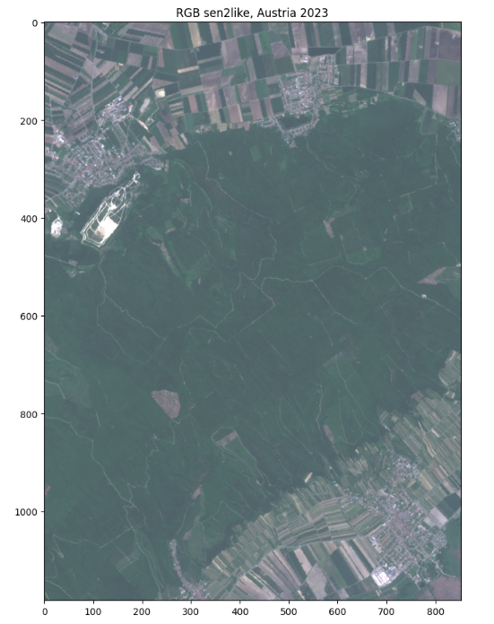
We select a temporal subset of the data to create an RGB. RGB stands for red (Band 4), green (Band 3), blue (Band 2) and describes the true colors of an image in remote sensing.
sen2_small = sen2like.filter_temporal(["2023-06-01", "2023-06-30"]).filter_bbox({"west": 16.6, "east": 16.7, "south": 47.9, "north": 48})
rgb = sen2_small.filter_bands(bands=["B02", "B03", "B04"])
We save the data into a NetCDF, a file format for storing multidimensional scientific data (variables). Two types of output are created: The Sen2Like original .SAFE files for the extent of four UTM tiles and the NetCDF for a smaller sector.
rgb_nc = rgb.save_result(format="NetCDF")
# 3. Running the Job
We create and start the openEO job. To reuse the results (e.g. for the indices notebook (opens new window)), we need to know the job id. To see the job status the job-variable has to be called.
job = rgb_nc.create_job().start_job()

job
Once the job status is "finished", we can download and explore the results.
results = job.get_results().download_files("sen2like_outputs")
# 4. Explore the openEO results
To create a plot of our data, we need the libraries numpy, xarray and matplotlib.pyplot. First, the desired data set must be selected.
import numpy as np
import xarray as xr
import matplotlib.pyplot as plt
path = "./sen2like_outputs/"
files = [path+file for file in os.listdir(path) if file.endswith(".nc")]
temp_xarray = []
for file in files:
    temp_xr = xr.open_dataset(file, chunks={})
    if "time" in temp_xr.coords:
        temp_xr = temp_xr.expand_dims("time")
    elif "t" in temp_xr.coords:
        temp_xr = temp_xr.expand_dims("t")
    temp_xarray.append(temp_xr)
data = xr.combine_by_coords(temp_xarray, fill_value=np.nan)

data = data.where(data!=-9999, np.nan)
data_t = data.isel(time=2)
To get a true color image the colors need to get adjusted. Then, we can plot our data.
brg = np.zeros((data_t.B04.shape[0],data_t.B04.shape[1],3))
brg[:,:,0] = (data_t.B04.values+1)/15
brg[:,:,1] = (data_t.B03.values+1)/14
brg[:,:,2] = (data_t.B02.values+1)/11.6
brg = np.clip(brg,0,255).astype(np.uint8)

plt.figure(figsize=(8,12))
plt.title("RGB sen2like, Austria 2023")
plt.imshow(brg,cmap='brg')
# 5. Indices calculations
To calculate some Indices on our L2F data, we’ve prepared another Jupyter Notebook (opens new window). We make use of the load_stac process, to reload the previously computed Sen2Like outputs. This is especially useful, when we compute multiple indices from the same Sen2Like outputs, as the Sen2Like processing only needs to be done once.
To load the results, insert the url with the saved "job_id" into the "load_stac" process. The spatio-temporal extent can be the same or smaller/shorter as in the selected data. We select the bands "B03", "B04", "B05", "B06", "B07", "B8A", "B11", "B12", as these are required in the computation for the following indices.
sen2like_job_id = "eodc-5d4c1746-33b2-42fb-914c-d36987747ae6"
spatial_extent = {"west": 16.6, "east": 16.7, "south": 47.9, "north": 48}
temporal_extent = ["2023-06-01", "2023-06-30"]
bands = ["B03", "B04", "B05", "B06", "B07", "B8A", "B11", "B12"]

data = conn.load_stac(
    url = f"https://openeo.eodc.eu/openeo/1.1.0/jobs/{sen2like_job_id}/results",
    spatial_extent=spatial_extent,
    temporal_extent=temporal_extent,
    bands=bands)
# 5.1 Leaf Area Index (LAI)
The LAI process is based on the computation specified at Sentinelhub (opens new window). All needed Bands and angles are included in the Sen2Like output data.
lai = data.process('lai', {'data': data})
lai_nc = lai.save_result(format="NetCDF", options={"tile_grid":"time-series"})
We create and start the openEO job. Once the job status is "finished", we can download the results.
job = lai_nc.create_job().start_job()
job.get_results().download_files("./lai/")
# 5.2 Leaf Chlorophyll Content (CAB)
With the same input as the LAI, the CAB can be calculated. The processing is based on the computation from Sentinelhub (opens new window).
cab = data.process('cab', {'data': data})
cab_nc = cab.save_result(format="NetCDF", options={"tile_grid":"time-series"})
job = cab_nc.create_job().start_job()
job.get_results().download_files("./cab/")
# 5.3 Fraction of green Vegetation Cover (FCOVER)
In the same manner, we compute the Fraction of green Vegetation Cover (FCOVER), which is based on the FCOVER-calculations from Sentinelhub (opens new window).
fcover = data.process('fcover', {'data': data})
fcover_nc = fcover.save_result(format="NetCDF", options={"tile_grid":"time-series"})
job = fcover_nc.create_job().start_job()
job.get_results().download_files("./fcover/")
# 5.4 Fraction of Absorbed Photosynthetically Active Radiation (FAPAR)
The FAPAR-computation can be found at Sentinelhub (opens new window).
fapar = data.process('fapar', {'data': data})
fapar_nc = fapar.save_result(format="NetCDF", options={"tile_grid":"time-series"})job = job = fapar_nc.create_job().start_job()
job.get_results().download_files("./fapar/")
# 5.5 Normalized difference vegetation index
The computation of the indices could also be done in one process graph with the Sen2Like processing. In this case, we start again with the "load_collection" process and select the bands "B04" and "B08".
spatial_extent =  {"west": 16.6, "east": 16.7, "south": 47.9, "north": 48}
temporal_extent = ["2023-06-01", "2023-09-30"]

collection      = 'SENTINEL2_L1C'
bands = ["B04", "B08"]

S2 = conn.load_collection(
    collection,
    spatial_extent=spatial_extent,
    temporal_extent=temporal_extent,
    bands=bands)


sen2like = S2.process('sen2like', {
    'data': THIS,
    'target_product': 'L2F',
    'export_original_files': True,
    'cloud_cover': 50})
We make use of the "ndvi" process and select a format and options for saving. Then we create and start the job and download the results.
ndvi = sen2like.ndvi(nir="B08", red="B04")
ndvi_nc = ndvi.save_result(format="NetCDF", options={"tile_grid":"time-series"})
job = ndvi_nc.create_job().start_job()
job.get_results().download_files("./ndvi/")
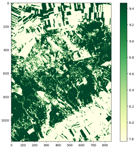
# 5.6 Explore the results
The functionality is shown using the LAI, but it works the same for the other indices. To create a plot of the results, we need the libraries os, numpy, mathplotlib and xarray. First, the LAI files are loaded. A map with the results is then created using matplotlib.pyplot.
import os
import numpy as np
import matplotlib.pyplot as plt
import xarray as xr

path = "./lai/"
files = [path+file for file in os.listdir(path) if file.startswith("Time")]
lai = xr.open_mfdataset(files).name
lai = lai.where(lai!=-9999, np.nan)
plt.figure(figsize=(10,8))
plt.imshow(lai[0], cmap="YlGn")
plt.colorbar()